In this tutorial, we’ll learn how to create heatmaps using gene expression data. Heatmaps are powerful visualization tools for gene expression data, allowing researchers to identify patterns, clusters, and differential expression across samples and genes. We will use the GEOquery package to download and process data from the Gene Expression Omnibus (GEO) database. Specifically, we will analyze the dataset with accession number GSE9723, which contains gene expression profiles of human gingival keratinocytes (HIGK) infected with two different bacteria.
Transcriptional profiling was utilized to define the biological pathways of gingival epithelial cells modulated by co-culture with the oral pathogenic Porphyromonas gingivalis and Aggregatibacter actinomycetemcomitans. We used microarrays to detail the global programme of gene expression underlying infection and identified distinct classes of up- and down-regulated genes during this process.
The files required for this analysis can be downloaded from GEO database. For quick access, The series matrix file for GSE9723 can be found here. This file contains the processed expression data along with sample annotations. The platform file for GPL96 can be found here. This file contains the probe annotations for the Affymetrix Human Genome U133A Array used in this study.
7.2 Installation of Required Packages
We will use the GEOquery package to read the series matrix file and extract the expression data and sample annotations. For processing differential expression, we will use the limma package. For preparing heatmaps, we will use two different packages — pheatmap and ComplexHeatmap. To install the required packages, use the following commands:
To read the series matrix file, we will use the getGEO function from the GEOquery package. The getGPL keyword argument is set to FALSE to avoid downloading the platform data, as we only need the expression data and sample annotations for this analysis. Subsequently, we will extract the expression data and phenotype data (sample annotations) from the GEO object using the exprs() and pData() functions respectively.
library(GEOquery)
Loading required package: Biobase
Loading required package: BiocGenerics
Attaching package: 'BiocGenerics'
The following objects are masked from 'package:stats':

    IQR, mad, sd, var, xtabs
Welcome to Bioconductor

    Vignettes contain introductory material; view with
    'browseVignettes()'. To cite Bioconductor, see
    'citation("Biobase")', and for packages 'citation("pkgname")'.
── Conflicts ────────────────────────────────────────── tidyverse_conflicts() ──
✖ dplyr::combine()    masks Biobase::combine(), BiocGenerics::combine()
✖ dplyr::filter()     masks stats::filter()
✖ dplyr::lag()        masks stats::lag()
✖ ggplot2::Position() masks BiocGenerics::Position(), base::Position()
ℹ Use the conflicted package (<http://conflicted.r-lib.org/>) to force all conflicts to become errors
library(gt)
Warning: package 'gt' was built under R version 4.4.3
# Read the series matrix file using GEOqueryseries_matrix_file <-"GEO_data_downloaded/GSE9723_series_matrix.txt"gse <-getGEO(filename = series_matrix_file, getGPL =FALSE)# Extract expression dataexpr_data <-exprs(gse)# Extract phenotype datapData <-pData(gse) %>%as_tibble(rownames ="sample_id")
7.4 Differential Expression Analysis
Next, using the limma package, we’ll identify differentially expressed genes (DEGs) between infected and control samples. We will create a design matrix based on the sample titles, fit a linear model, and apply empirical Bayes moderation to obtain the DEGs, and extract the top 50 DEGs for further analysis.
library(limma)
Attaching package: 'limma'
The following object is masked from 'package:BiocGenerics':

    plotMA
# Create design matrixgroup_factor <-factor(ifelse(grepl("Sham", pData$title, ignore.case =TRUE), "Control", "Infected"))design <-model.matrix(~0+ group_factor)colnames(design) <-make.names(levels(group_factor))# Run limmafit <-lmFit(expr_data, design)contrast_matrix <-makeContrasts(Infected - Control, levels = design)fit2 <-contrasts.fit(fit, contrast_matrix)fit2 <-eBayes(fit2)# Get top DEGsdeg <-topTable(fit2, adjust ="fdr", number =Inf)top_degs <-rownames(deg)[1:50]# Read platform annotation file to map probe IDs to gene symbolsplatform_file <-"GEO_data_downloaded/GPL96-57554.txt"platform_data <-read.delim(platform_file, sep ="\t", skip =16, header =TRUE,stringsAsFactors =FALSE, comment.char ="#")# Create a mapping from probe ID to gene symbolprobe_to_gene <- platform_data %>%select(ID, Gene.Symbol) %>%mutate(Gene.Symbol =ifelse(Gene.Symbol =="", NA, Gene.Symbol)) %>%deframe()# Add gene symbols to deg tabledeg_with_genes <- deg %>%as.data.frame() %>%rownames_to_column("ProbeID") %>%mutate(Gene = probe_to_gene[ProbeID]) %>%mutate(Gene =ifelse(is.na(Gene), ProbeID, Gene))# Display top 10 with gene symbolshead(deg_with_genes[, c("Gene", "logFC", "adj.P.Val")], 10) %>%gt() %>%tab_header(title ="Top 10 Differentially Expressed Genes")
Top 10 Differentially Expressed Genes
Gene
logFC
adj.P.Val
SNAI2
-2508.6750
0.005145103
IL1B
3268.4125
0.005145103
ZFP36L1
-685.6500
0.015821475
TMEM127
-205.4250
0.019209550
BUD31
-364.8375
0.019209550
PPP2R2D
-117.5250
0.019209550
TNFRSF12A
-2173.4750
0.019209550
FARS2
-45.0125
0.022918236
DIEXF
158.2125
0.026242237
INO80D
99.8000
0.029204904
7.5 Sample Information
pData %>%select(sample_id, title, status, treatment_protocol_ch1) %>%gt() %>%tab_header(title ="Sample Information for GSE9723") %>%tab_options(container.height ="50vh")
Sample Information for GSE9723
sample_id
title
status
treatment_protocol_ch1
GSM245725
HIGK cells infected with Porphyromonas gingivalis, biological rep1
Public on Apr 15 2008
Bacteria at mid-log phase were harvested and washed by centrifugation, and resuspended in antibiotic-free K-SFM media. HIGK cells (10e7) were co-cultured with bacteria to give a total association (adhered plus invaded) of approximately 100 organisms per epithelial cell. Numbers of adhered and invaded organisms were confirmed in parallel experiments by plate counting. After 2 hours at 37C in 5% CO2, the HIGK cells were lysed with Trizol (Invitrogen) prior to RNA extraction.
GSM245726
HIGK cells infected with Porphyromonas gingivalis, biological rep2
Public on Apr 15 2008
Bacteria at mid-log phase were harvested and washed by centrifugation, and resuspended in antibiotic-free K-SFM media. HIGK cells (10e7) were co-cultured with bacteria to give a total association (adhered plus invaded) of approximately 100 organisms per epithelial cell. Numbers of adhered and invaded organisms were confirmed in parallel experiments by plate counting. After 2 hours at 37C in 5% CO2, the HIGK cells were lysed with Trizol (Invitrogen) prior to RNA extraction.
GSM245727
HIGK cells infected with Porphyromonas gingivalis, biological rep3
Public on Apr 15 2008
Bacteria at mid-log phase were harvested and washed by centrifugation, and resuspended in antibiotic-free K-SFM media. HIGK cells (10e7) were co-cultured with bacteria to give a total association (adhered plus invaded) of approximately 100 organisms per epithelial cell. Numbers of adhered and invaded organisms were confirmed in parallel experiments by plate counting. After 2 hours at 37C in 5% CO2, the HIGK cells were lysed with Trizol (Invitrogen) prior to RNA extraction.
GSM245728
HIGK cells infected with Porphyromonas gingivalis, biological rep4
Public on Apr 15 2008
Bacteria at mid-log phase were harvested and washed by centrifugation, and resuspended in antibiotic-free K-SFM media. HIGK cells (10e7) were co-cultured with bacteria to give a total association (adhered plus invaded) of approximately 100 organisms per epithelial cell. Numbers of adhered and invaded organisms were confirmed in parallel experiments by plate counting. After 2 hours at 37C in 5% CO2, the HIGK cells were lysed with Trizol (Invitrogen) prior to RNA extraction.
GSM245729
Sham infected HIGK cells, biological rep1 (1777)
Public on Mar 01 2008
HIGK cells were sham infected with antibiotic-free K-SFM media. HIGK cells (10e7) were cultured for 2 hours at 37C in 5% CO2, and were lysed with Trizol (Invitrogen) prior to RNA extraction.
GSM245730
Sham infected HIGK cells, biological rep2 (1778)
Public on Mar 01 2008
HIGK cells were sham infected with antibiotic-free K-SFM media. HIGK cells (10e7) were cultured for 2 hours at 37C in 5% CO2, and were lysed with Trizol (Invitrogen) prior to RNA extraction.
GSM245731
Sham infected HIGK cells, biological rep3 (1779)
Public on Mar 01 2008
HIGK cells were sham infected with antibiotic-free K-SFM media. HIGK cells (10e7) were cultured for 2 hours at 37C in 5% CO2, and were lysed with Trizol (Invitrogen) prior to RNA extraction.
GSM245732
Sham infected HIGK cells, biological rep4 (1780)
Public on Mar 01 2008
HIGK cells were sham infected with antibiotic-free K-SFM media. HIGK cells (10e7) were cultured for 2 hours at 37C in 5% CO2, and were lysed with Trizol (Invitrogen) prior to RNA extraction.
GSM245733
HIGK cells infected with Aggregatibacter actinomycetemcomitans, biological rep1
Public on Mar 01 2008
Bacteria at mid-log phase were harvested and washed by centrifugation, and resuspended in antibiotic-free K-SFM media. HIGK cells (10e7) were co-cultured with bacteria to give a total association (adhered plus invaded) of approximately 2500 organisms per epithelial cell. Numbers of adhered and invaded organisms were confirmed in parallel experiments by plate counting. After 2 hours at 37C in 5% CO2, the HIGK cells were lysed with Trizol (Invitrogen) prior to RNA extraction.
GSM245734
HIGK cells infected with Aggregatibacter actinomycetemcomitans, biological rep2
Public on Mar 01 2008
Bacteria at mid-log phase were harvested and washed by centrifugation, and resuspended in antibiotic-free K-SFM media. HIGK cells (10e7) were co-cultured with bacteria to give a total association (adhered plus invaded) of approximately 2500 organisms per epithelial cell. Numbers of adhered and invaded organisms were confirmed in parallel experiments by plate counting. After 2 hours at 37C in 5% CO2, the HIGK cells were lysed with Trizol (Invitrogen) prior to RNA extraction.
GSM245735
HIGK cells infected with Aggregatibacter actinomycetemcomitans, biological rep3
Public on Mar 01 2008
Bacteria at mid-log phase were harvested and washed by centrifugation, and resuspended in antibiotic-free K-SFM media. HIGK cells (10e7) were co-cultured with bacteria to give a total association (adhered plus invaded) of approximately 2500 organisms per epithelial cell. Numbers of adhered and invaded organisms were confirmed in parallel experiments by plate counting. After 2 hours at 37C in 5% CO2, the HIGK cells were lysed with Trizol (Invitrogen) prior to RNA extraction.
GSM245736
HIGK cells infected with Aggregatibacter actinomycetemcomitans, biological rep4
Public on Mar 01 2008
Bacteria at mid-log phase were harvested and washed by centrifugation, and resuspended in antibiotic-free K-SFM media. HIGK cells (10e7) were co-cultured with bacteria to give a total association (adhered plus invaded) of approximately 2500 organisms per epithelial cell. Numbers of adhered and invaded organisms were confirmed in parallel experiments by plate counting. After 2 hours at 37C in 5% CO2, the HIGK cells were lysed with Trizol (Invitrogen) prior to RNA extraction.
7.6 Heatmap using pheatmap
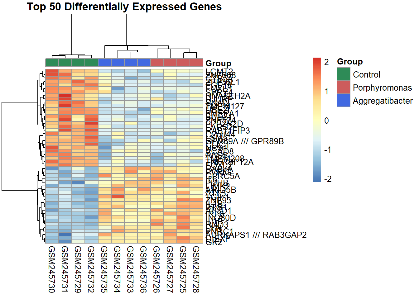
For our heatmap, we need to create an annotation data frame that categorizes samples based on the bacteria they were infected with. So we’ll add a new Group column to the phenotype data, which will classify samples into “Control”, “Porphyromonas”, and “Aggregatibacter” groups based on the sample titles. For the heatmap, the data source will be the expression values of the top 50 DEGs identified earlier. The scale = "row" argument will standardize the expression values for each gene across all samples, allowing us to visualize relative expression levels. In the heatmap, clustering of both rows (genes) and columns (samples) will be performed using correlation distance to group similar expression patterns together.
# Create annotation with specific bacteria names from titlesample_groups_detailed <- pData %>%mutate(Group =case_when(grepl("Sham", title, ignore.case =TRUE) ~"Control",grepl("Porphyromonas", title, ignore.case =TRUE) ~"Porphyromonas",grepl("Aggregatibacter", title, ignore.case =TRUE) ~"Aggregatibacter",TRUE~"Other" )) %>%pull(Group)annotation_df <-data.frame(Group =factor(sample_groups_detailed),row.names =colnames(expr_data))# Define custom colors for annotationannotation_colors <-list(Group =c("Control"="#2E8B57", "Porphyromonas"="#CD5C5C", "Aggregatibacter"="#4169E1"))# Generate heatmap using top DEGs# Create expression matrix with gene symbols as row namesexpr_heatmap <- expr_data[top_degs, ]rownames(expr_heatmap) <- probe_to_gene[rownames(expr_heatmap)]# If any gene symbols are NA, keep the original probe IDrownames(expr_heatmap) <-ifelse(is.na(rownames(expr_heatmap)), top_degs, rownames(expr_heatmap))pheatmap(expr_heatmap,scale ="row",annotation_col = annotation_df,annotation_colors = annotation_colors,show_rownames =TRUE,show_colnames =TRUE,clustering_distance_rows ="correlation",clustering_distance_cols ="correlation",main ="Top 50 Differentially Expressed Genes")
7.7 Clustering Distance Metrics options
When creating heatmaps, choosing the right clustering parameters is crucial for revealing meaningful patterns in the data.
7.7.1 Distance Metrics in pheatmap
Distance Metric
Best For
Description
"euclidean"
Absolute expression differences
Straight-line distance between expression vectors. Good when magnitude matters.
"correlation"
Shape of expression patterns
Pearson correlation. Ideal for gene expression where co-regulation matters more than absolute values. Internally, it calculates distance as \[ d = 1 - correlation \]
"manhattan"
High-dimensional data
Sum of absolute differences. Less sensitive to outliers than Euclidean.
"maximum"
Outlier robustness
Maximum coordinate difference
"canberra"
Sparse data
Weighted Manhattan distance
"minkowski"
Generalized distance
Generalization of Euclidean and Manhattan
"binary"
Presence/absence data
For binary matrices
Note: pheatmap uses base R’s dist() function. For Spearman correlation, pre-calculate the distance matrix using as.dist(1 - cor(t(expr_matrix), method = "spearman")) and pass it to the clustering_distance_rows parameter.
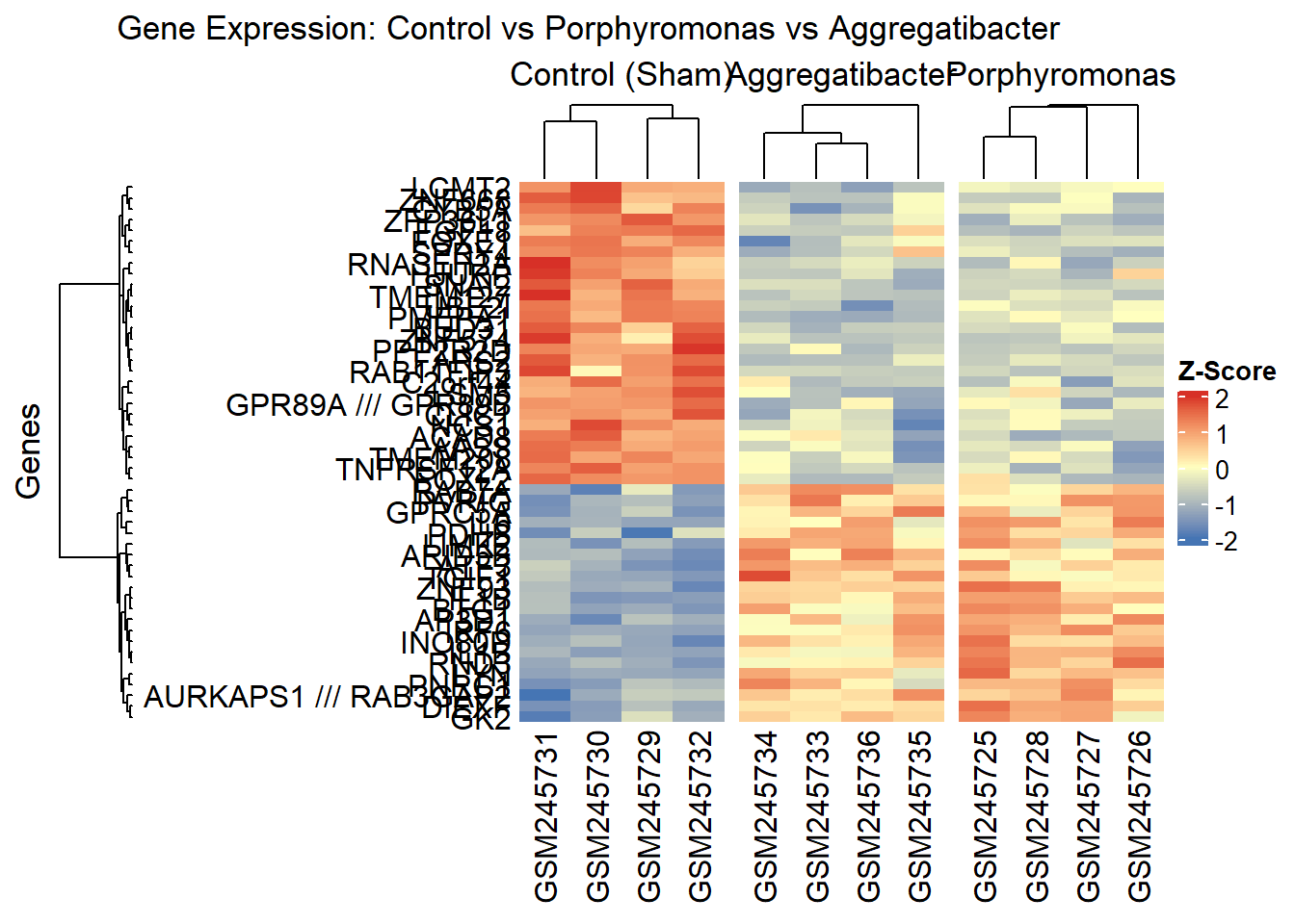
7.8 Heatmap using ComplexHeatmap
Bioconductor has another powerful package for creating heatmaps called ComplexHeatmap. We’ll use the same dataset as before, but this time we’ll create three separate heatmaps for each group: Control (Sham), Porphyromonas infected, and Aggregatibacter infected samples. And then make one combined heatmap showing all three groups side by side for comparison. Note that with ComplexHeatmap, we need to manually scale the data by row (z-score) since it doesn’t have a built-in scaling option like pheatmap. This might look as extra work, but it gives us more control over the scaling process e.g. choosing a different method of scaling if needed and handling missing values more flexibly.
library(ComplexHeatmap)
Loading required package: grid
========================================
ComplexHeatmap version 2.22.0
Bioconductor page: http://bioconductor.org/packages/ComplexHeatmap/
Github page: https://github.com/jokergoo/ComplexHeatmap
Documentation: http://jokergoo.github.io/ComplexHeatmap-reference

If you use it in published research, please cite either one:
- Gu, Z. Complex Heatmap Visualization. iMeta 2022.
- Gu, Z. Complex heatmaps reveal patterns and correlations in multidimensional
    genomic data. Bioinformatics 2016.


The new InteractiveComplexHeatmap package can directly export static
complex heatmaps into an interactive Shiny app with zero effort. Have a try!

This message can be suppressed by:
  suppressPackageStartupMessages(library(ComplexHeatmap))
========================================
! pheatmap() has been masked by ComplexHeatmap::pheatmap(). Most of the arguments
   in the original pheatmap() are identically supported in the new function. You
   can still use the original function by explicitly calling pheatmap::pheatmap().
Attaching package: 'ComplexHeatmap'
The following object is masked from 'package:gt':

    row_order
The following object is masked from 'package:pheatmap':

    pheatmap
library(circlize)
Warning: package 'circlize' was built under R version 4.4.3
========================================
circlize version 0.4.17
CRAN page: https://cran.r-project.org/package=circlize
Github page: https://github.com/jokergoo/circlize
Documentation: https://jokergoo.github.io/circlize_book/book/

If you use it in published research, please cite:
Gu, Z. circlize implements and enhances circular visualization
  in R. Bioinformatics 2014.

This message can be suppressed by:
  suppressPackageStartupMessages(library(circlize))
========================================
# Get sample groups with bacteria namessample_groups_detailed <- pData %>%mutate(Group =case_when(grepl("Sham", title, ignore.case =TRUE) ~"Control",grepl("Porphyromonas", title, ignore.case =TRUE) ~"Porphyromonas",grepl("Aggregatibacter", title, ignore.case =TRUE) ~"Aggregatibacter",TRUE~"Other" )) %>%pull(Group)# Split samples into groupscontrol_samples <-colnames(expr_data)[sample_groups_detailed =="Control"]porphyromonas_samples <-colnames(expr_data)[sample_groups_detailed =="Porphyromonas"]aggregatibacter_samples <-colnames(expr_data)[sample_groups_detailed =="Aggregatibacter"]# Use top DEGs# Check which top DEGs are in the expression matrixavailable_degs <- top_degs[top_degs %in%rownames(expr_data)]if (length(available_degs) ==0) {# If no match, use numeric indices available_degs <-rownames(expr_data)[as.numeric(top_degs)] available_degs <- available_degs[!is.na(available_degs)]}# Scale data by row (z-score) - same as pheatmap scale="row"expr_scaled <-t(apply(expr_data[available_degs, ], 1, function(x) { (x -mean(x, na.rm =TRUE)) /sd(x, na.rm =TRUE)}))# Replace probe IDs with gene symbols for row namesrownames(expr_scaled) <- probe_to_gene[rownames(expr_scaled)]# If any gene symbols are NA, keep the original probe IDrownames(expr_scaled) <-ifelse(is.na(rownames(expr_scaled)), available_degs, rownames(expr_scaled))# Define color scheme - matching pheatmap default (blue-white-red)col_fun <-colorRamp2(c(-2, 0, 2), c("#4575B4", "#FFFFBF", "#D73027"))# Calculate row clustering using ALL samples (matching pheatmap behavior)# Create distance matrix and dendrogram for rows using correlationrow_dist <-as.dist(1-cor(t(expr_scaled)))row_dend <-hclust(row_dist, method ="complete")# Create heatmap for Control samplesht_control <-Heatmap(expr_scaled[, control_samples],name ="Expression",col = col_fun,column_title ="Control (Sham)",row_title ="Genes",cluster_rows = row_dend, # Use dendrogram based on all samplescluster_columns =TRUE,clustering_distance_columns ="pearson",show_row_names =TRUE,row_names_side ="left",row_dend_side ="left",show_column_names =TRUE,show_heatmap_legend =TRUE,heatmap_legend_param =list(title ="Z-Score"))# Create heatmap for Porphyromonas infected samplesht_porphyromonas <-Heatmap(expr_scaled[, porphyromonas_samples],col = col_fun,column_title ="Porphyromonas",cluster_rows = row_dend, # Same row order as controlcluster_columns =TRUE,clustering_distance_columns ="pearson",show_row_names =FALSE,show_column_names =TRUE,show_heatmap_legend =FALSE)# Create heatmap for Aggregatibacter infected samplesht_aggregatibacter <-Heatmap(expr_scaled[, aggregatibacter_samples],col = col_fun,column_title ="Aggregatibacter",cluster_rows = row_dend, # Same row order as controlcluster_columns =TRUE,clustering_distance_columns ="pearson",show_row_names =FALSE,show_column_names =TRUE,show_heatmap_legend =FALSE)# Combine heatmaps horizontallyht_combined <- ht_control + ht_aggregatibacter + ht_porphyromonasdraw(ht_combined, column_title ="Gene Expression: Control vs Porphyromonas vs Aggregatibacter")
7.8.1 Distance Metrics in ComplexHeatmap
ComplexHeatmap supports all pheatmap distances plus some additional options for correlation-based distances.