library(tidyverse)
library(ggsignif)2 t_test
2.1 Introduction
A t-test is a statistical test used to compare the means of two groups to check if they are significantly different from each other. A t-test can be one sample t-test where we compare the mean of a group to a known or hypothesized value. The more commonly used t-test is two-sample t-test where we compare means between the two groups. These can be further divided into two categories.
1) Independent-samples (two-sample) T-test: The means of two independent groups are check. E.g. means of a measurement from control group and treatment group.
2) Paired-samples (dependent-samples) T-test: The means of two related groups are compared. E.g. means of a measurement before and after treatment for the same group.
2.2 Formula for independent t-test
\[ t = \frac{\bar{x_1} - \bar{x_2}}{\sqrt{\frac{s_{1}^2}{n_1} + \frac{s_{2}^2}{n_2}}} \]
where, \(\bar{x_1}\) and \(\bar{x_2}\) are sample means, \(s_{1}^2\) and \(s_{2}^2\) are sample variances, and \(n_1\) and \(n_2\) are sample sizes.
The t-value is then compared to a critical value from the t-distribution (based on degrees of freedom) to determine statistical significance denoted using a p-value.
2.3 Dataset
For the learning t-test, we will use the data from the paper:
Isoprene deters insect herbivory by priming plant hormone responses
Our objective is to re-create figure 1b from the paper. The data for figure 1b is available as supplementary information and can be download from here.
Read the data into R using the read.csv function. The first two rows are just additional information, so we will skip them using the skip argument. Also, the last 3 row are summary statistics, so we will remove them using the slice function from the dplyr package.
fly_data <- read.csv("../data_viz/Fig_1b.csv", skip = 2)

# keep only the first 15 rows using dplyr
fly_data <- fly_data %>%
  slice(1:15)

colnames(fly_data)
[1] "Sample" "Area..cm2."
[3] "No..of.white.flies" "No..of.white.flies..cm.2"
[5] "Sample.1" "Area..cm.2."
[7] "No..of.white.flies.1" "No..of.white.flies..cm.2.1"2.4 t-test
The data has two columns with the number of white flies per cm2 for two different conditions. We will use the t.test function to perform a t-test on these two columns. The paired argument is set to FALSE because the two groups are independent.
The t.test function returns a list of values including the t-value, degrees of freedom, confidence interval, and p-value. The p-value is used to determine if the difference between the two groups is statistically significant.
t_test_result <- t.test(fly_data$No..of.white.flies..cm.2, fly_data$No..of.white.flies..cm.2.1, paired = F)
t_test_result
    Welch Two Sample t-test

data:  fly_data$No..of.white.flies..cm.2 and fly_data$No..of.white.flies..cm.2.1
t = 2.9909, df = 19.835, p-value = 0.007268
alternative hypothesis: true difference in means is not equal to 0
95 percent confidence interval:
 0.157744 0.886256
sample estimates:
mean of x mean of y
0.8153333 0.2933333
2.5 Plotting
We will use the ggplot2 package to create a boxplot of the two groups using geom_boxplot function. Next, we’ll add individual data points to the plot using the geom_jitter function.
We could use the t_test_result object to add the t-test results to the plot, however it is easier to use the geom_signif function from the ggsignif package. This function allows us to add significance asterisks to the plot.
Finally, we’ll do some formatting of the plot using the theme, labs, and scale_* functions so that it looks similar to the figure in the paper.
fly_data %>%
  pivot_longer(cols = c(No..of.white.flies..cm.2, No..of.white.flies..cm.2.1),
               names_to = "Condition", values_to = "Count") %>%
  ggplot(aes(x = Condition, y = Count))+ #color = Condition)) +
  geom_boxplot(outlier.colour = NA, width=0.5, fill="lightgrey") +
  geom_jitter(color = 'black', width = 0.2, shape=1, size=3) +
#  geom_jitter(aes(color = Condition), width = 0.2, shape=1, size=3) +
  geom_signif(comparisons = list(c("No..of.white.flies..cm.2", "No..of.white.flies..cm.2.1")),
              test='t.test', map_signif_level = TRUE,
              tip_length=c(0.05,0.5), textsize=6,
              size=0.5, y_position = 2.75, vjust=1.75) +
  theme_minimal() +
  # scale y axis from 0 to 3
  scale_y_continuous(limits = c(0, 3), breaks = seq(0,3)) +
  scale_x_discrete(labels = c("NE", "IE")) +
  labs(x = element_blank(),
       y = expression("No. of white flies/cm"^2)) +
  # remove legend
  theme(legend.position = "none",
        panel.grid.major = element_blank(),
        panel.grid.minor = element_blank(),
        panel.border = element_rect(fill = NA, color = "black", linewidth = 1),
        axis.ticks.length = unit(0.2, "cm"),
        axis.ticks = element_line(color = "black", linewidth = 0.5))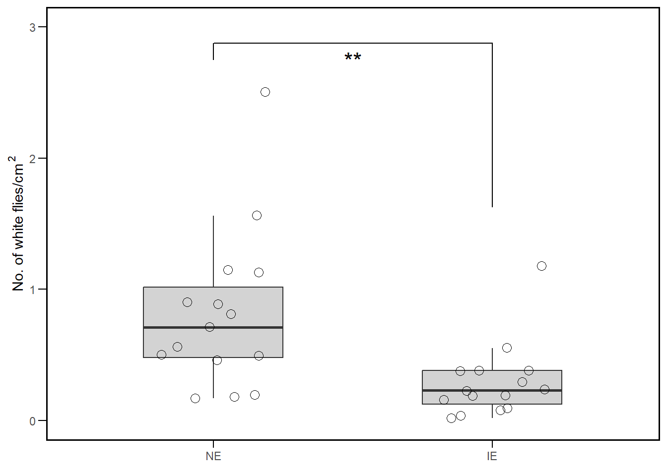
# save the plot
ggsave("../data_viz/Fig_1b.png", width = 5, height = 4,bg="white", dpi = 300)