6 Phylogenetic Trees

6.1 Introduction

One of the fundamental tasks in biology is to understand the relationship between different species or genes. A Phylogenetic tree is a diagram that represents such relationships. There are many program that can construct a phylogenetic tree given a set of multiple sequence alignments. The ggtree package in R is a powerful tool for visualizing and annotating phylogenetic trees. As the name suggest, it expands the capabilities of the ggplot2 package to visualize tree data.

To install this pacakage, run the following command:

BiocManager::install("ggtree")

Now load the ggplot2 and ggtree packages. Also, treeio package is required to read the tree files.

library("ggplot2")
library("treeio")
library("ggtree")

6.2 Read a tree file

One of the common format to store a phylogenetic tree is the Newick format. The Newick format is a way of representing a tree structure in a plain text format. For example, following is a simple Newick format tree - ((A,B),C). In this example, A and B are the two nodes in the tree which belong to the same clade, and C is a separate node.

The Newick format can also include branch lengths, which are represented by numbers after the node names. For example, ((A:0.1,B:0.2):0.3,C:0.4) represents a tree where A and B are in the same clade, and C is a separate node with branch lengths of 0.1, 0.2, 0.3, and 0.4 respectively.

We can read a phylogenetic tree in a Newick format using the read.tree function from the treeio package as shown below.

tree <- read.tree("dhfr_20.tree")
str(tree)

List of 4
 $ edge       : int [1:37, 1:2] 21 22 23 24 25 26 27 28 29 30 ...
 $ edge.length: num [1:37] 0.0107 0.0196 0.0387 0.129 0.0412 ...
 $ Nnode      : int 18
 $ tip.label  : chr [1:20] "sp|P37508|YYAP_BACSU" "sp|Q04515|DYR10_ECOLX" "sp|Q5V3R2|DYR1_HALMA" "sp|Q93341|DYR_CAEEL" ...
 - attr(*, "class")= chr "phylo"
 - attr(*, "order")= chr "cladewise"

If we look at the structure of the tree object, we can see that it contains four lists:

List Name	Description
`edge`	A matrix containing the edges of the tree. Each row represents an edge, and the columns represent the parent and child nodes of the edge.
`edge.length`	A vector that contains the lengths of the edges.
`Nnode`	Number of nodes in the tree.
`tip.label`	A vector that contains the node labels

We can access individual lists using the $ operator. For example, to get the number of nodes in the tree, use tree$Nnode.

6.3 Tree visualization

To visualize a phylogenetic tree, we can use the ggtree function from the ggtree package. The ggtree package is built on top of the ggplot2 package and provides a set of functions to visualize and annotate phylogenetic trees.

The ggtree function takes a phylogenetic tree object as an argument and returns a ggplot object that can be further customized using the ggplot2 functions. For instance, to show the node labels we can add a geom_tiplab layer to the plot.

ggtree(tree) + geom_tiplab()

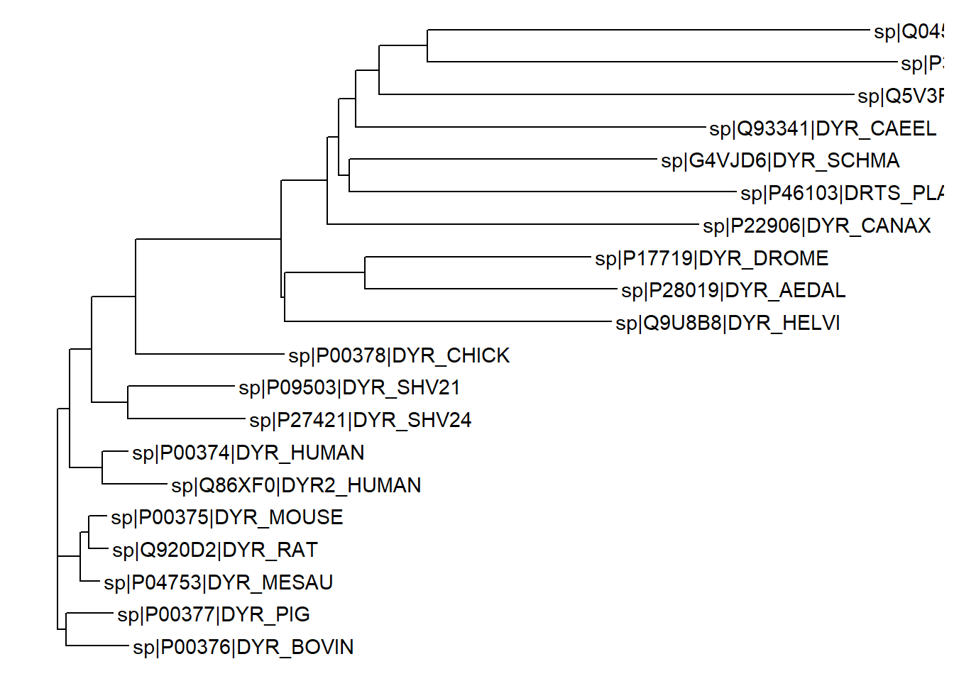
The ggtree function also provides several options to customize the appearance of the phylogenetic tree. To customize the branch color and thinkness, we can use the color and size arguments in the ggtree function. In addition, we can also change the color of the node labels by adding the color argument to the geom_tiplab function.

ggtree(tree, color="firebrick", size=1) + geom_tiplab(color="purple")

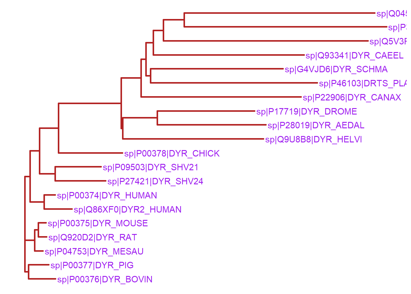
Furthermore, the node points and tip points can be customized using the geom_nodepoint and geom_tippoint functions respectively, as shown below.

ggtree(tree, ladderize=FALSE) +
   geom_nodepoint(color="blue", alpha=1/4, size=4) +
  geom_tippoint(color="#FDAC4F", shape=8, size=2) + 
  geom_tiplab(size=3, color="brown")

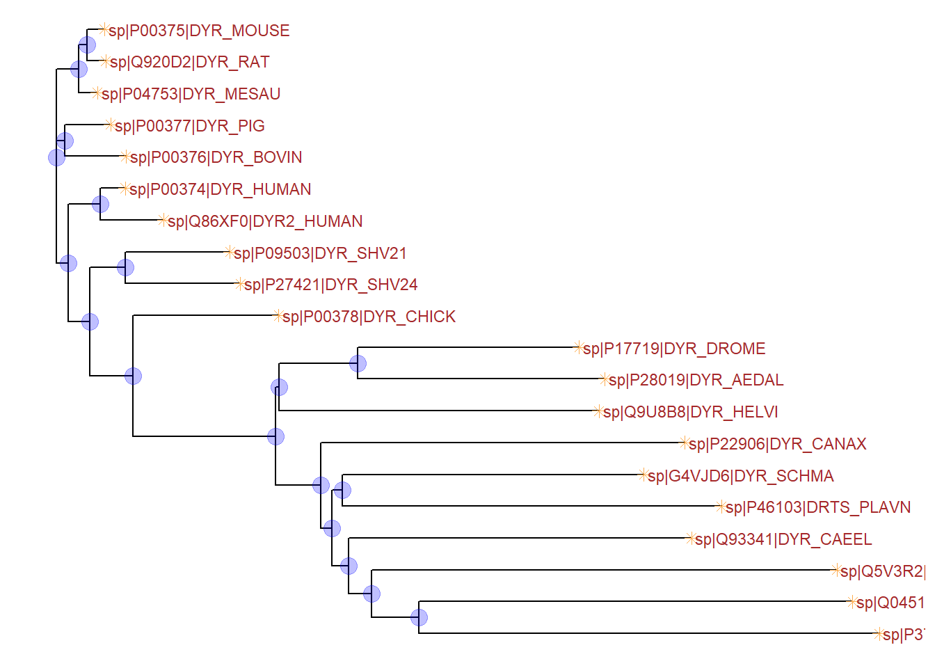
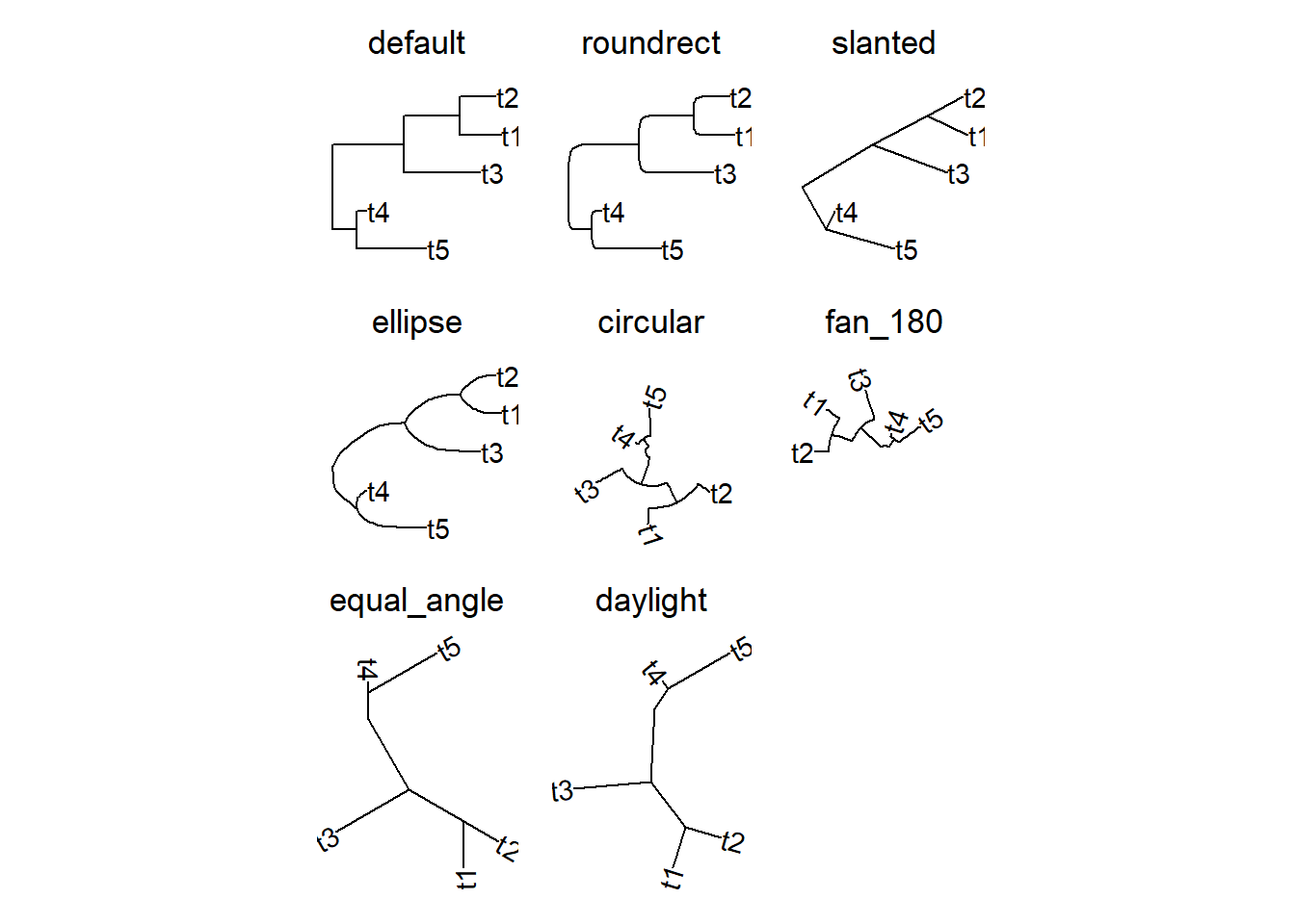
6.4 Tree layouts

With the ggtree package, we can visualize the phylogenetic tree in different layouts. The layout argument in the ggtree function allows us to specify the layout of the tree. The figure below shows the layout options.

6.5 Customizing node labels

We can edit the tree object to customize the rendering of the tree. For instance, we can access the node labels using the tree$tip.label and then edit these as required. The code below shows the use of the str_split_fixed function from the stringr package to split the node labels into three parts using the pipe character as a delimiter. The third part of the split is then used as the new node label after re-assigning the labels to the tree$tip.label list. This way, the labels now have the protein name only and the database identifier along with accession number are removed (compare the labels with the tree above).

library(stringr)
tree <- read.tree("dhfr_20.tree")
tree$tip.label <- str_split_fixed(tree$tip.label, "\\|",3)[, 3]

ggtree(tree, layout = "ellipse") + geom_tiplab() + 
  xlim(0,1)

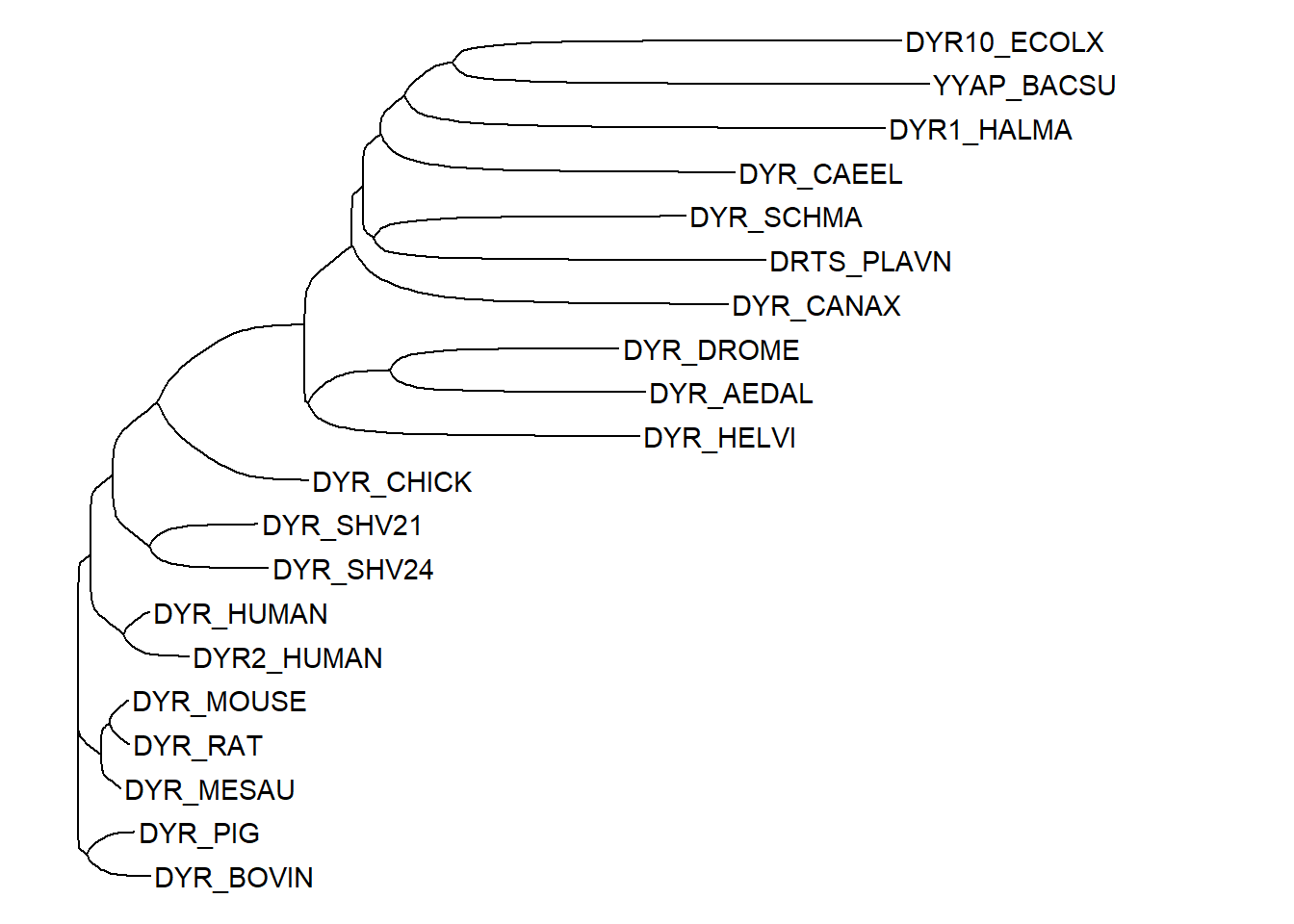
6.6 Highlight clades

To view a specific clade in the tree, the viewClade can be used. This function takes a ggtree object and a node number as arguments and returns a new ggtree object. The node number can be obtained using the MRCA function. The MRCA function takes a tree object and two or more node labels as arguments and returns the most recent common ancestor (MRCA) of the specified nodes. The code below show the clade correponding to the two nodes i.e. DYR10_ECOLX and DYR_CANAX.

viewClade(ggtree(tree) + geom_tiplab(), MRCA(tree,"DYR10_ECOLX", "DYR_CANAX"))

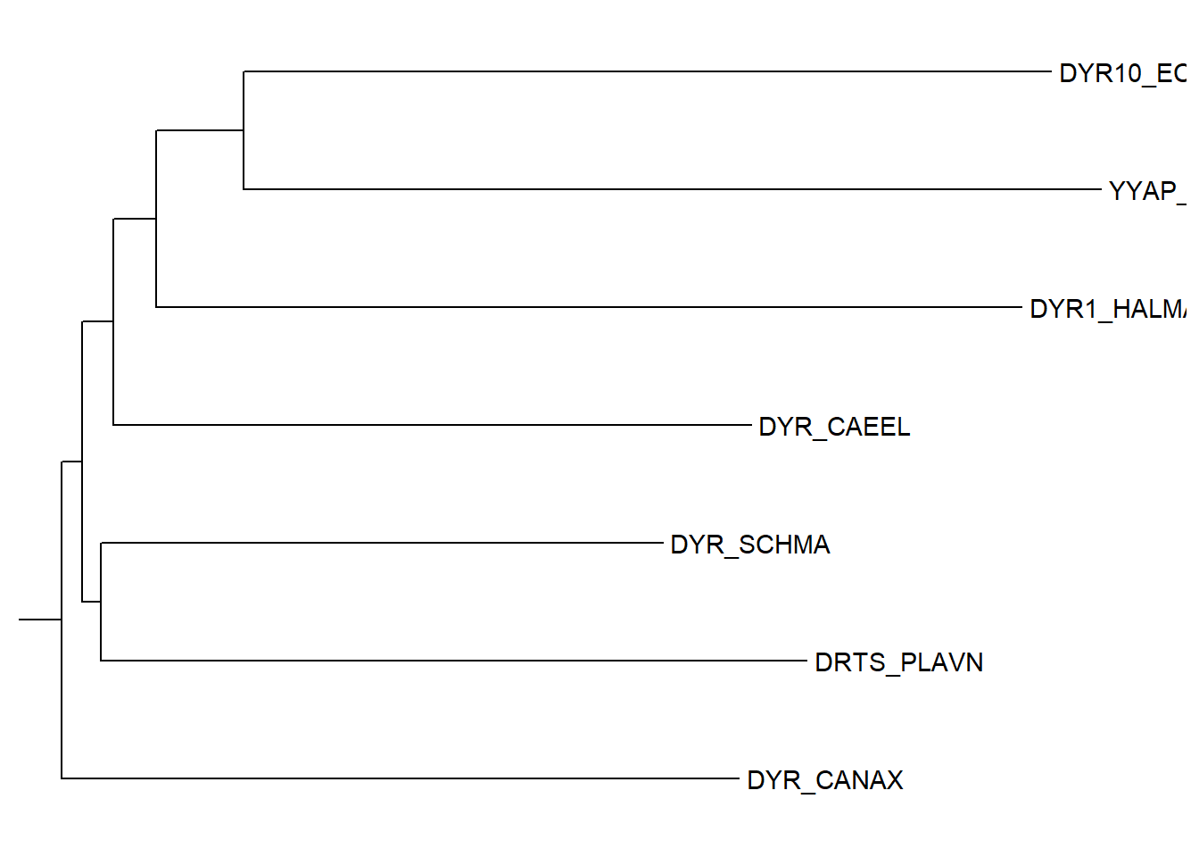
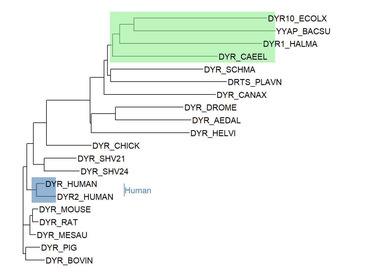
We can also highlight the clade using the geom_hilight function. The geom_hilight function takes a node number and a fill color as arguments. An MRCA object can be used to specify the node number. The code below shows highlighting of two clades - 1) for the MRCA of DYR10_ECOLX and DYR_CANAX and 2) for human sequences. A clade label can be optionally added as well.

ggtree(tree) + 
    geom_hilight(node=35, fill="steelblue", alpha=.6) +
    geom_hilight(node=MRCA(tree, .node1 =c("DYR_CAEEL", "DYR10_ECOLX")), 
                 fill="lightgreen", alpha=.6) + 
    geom_tiplab() + 
    geom_cladelabel(node=35, label="Human", color="steelblue", offset = 0.2) +
  xlim(0, 1)