library(readxl)
library(tidyverse)
library(multcomp)3 ANOVA
3.1 Introduction
ANalysis Of VAriance (ANOVA) is a statistical method to test whether there are significant differences between the means of three or more groups. It has two main types:
1) One-way ANOVA: Tests differences between groups based on one independent variable.
2) Two-way ANOVA: Considers two independent variables.
3.2 ANOVA in R
To learn how to perform ANOVA in R, we will use the data from the paper:
The data is available in the supplementary materials of the paper (link).
Here, we’ll reproduce the results from Figure 3c of the manuscript.
The data for Figure 3 is in the sheet 3 of the Excel file. We’ll skip the first row which just contains some header information. Also we need data from the first six columns (A-F). To read the excel file we’ll use read_excel function from the readxl package.
After creating the dataframe LH_gamma, we will convert the Genotype column to a factor since this will be required for the subsequent ANOVA analysis.
LH_gamma <- read_excel("plos_bio1.xlsx", sheet=3, range="A2:F39")

LH_gamma_2 <- LH_gamma %>%
  mutate(Genotype = factor(Genotype, levels = c("Control", "EC-Tau", "hAPP", "EC-Tau/hAPP")))
To perform ANOVA, we will use the aov function. For our analysis we want to test the null hypothesis that the means of the four Genotypes are equal. The independent varialbe is Theta (4-12 Hz) % and the dependent variable is Genotype. So, the formula for the ANOVA is: Theta (4-12 Hz) % ~ Genotype
Next, we will use the glht function from the multcomp package to perform post-hoc analysis. glht stands for “general linear hypothesis test”. The glht function takes the ANOVA results and the type of post-hoc test as arguments. In our case, we will use Dunnett’s test to compare each group with the control group. The mcp function is used to specify the type of comparison.
By default the first group is considered as the control group. If you want to change the control group, you can use the control argument in the mcp function.
anova_results <- aov(`Theta (4-12 Hz) %` ~ Genotype, data=LH_gamma_2)
dunnett_results <- glht(anova_results, linfct = mcp(Genotype = "Dunnett"))
summary_dunnett <- summary(dunnett_results)
summary_dunnett
     Simultaneous Tests for General Linear Hypotheses

Multiple Comparisons of Means: Dunnett Contrasts


Fit: aov(formula = `Theta (4-12 Hz) %` ~ Genotype, data = LH_gamma_2)

Linear Hypotheses:
                           Estimate Std. Error t value Pr(>|t|)
EC-Tau - Control == 0        -7.128      6.176  -1.154  0.52349
hAPP - Control == 0         -15.961      5.840  -2.733  0.02666 *
EC-Tau/hAPP - Control == 0  -19.185      5.840  -3.285  0.00667 **
---
Signif. codes:  0 '***' 0.001 '**' 0.01 '*' 0.05 '.' 0.1 ' ' 1
(Adjusted p values reported -- single-step method)
3.3 Preparing the data for plotting
Based on the p-values for the pairwise comparison, a stars variable is created to hold the significance level of each comparison. The cut function is used to create a categorical variable based on the p-values stored in p_values variable. The breaks argument specifies the cut points for the categories, and the labels argument specifies the labels for each category.
The names for the pair of groups being compared are stored in the pair_names variable. These names can be accessed using the names function on the summary_dunnett$test$tstat object.
The LH_gamma_summarydataframe is created using the group_by and summarise functions from the dplyr package. The mean_theta and sem_theta (standard error of the mean) are calculated for each Genotype group.
p_values <- summary_dunnett$test$pvalues
stars <- cut(p_values,
             breaks = c(-Inf, 0.001, 0.01, 0.05, 1),
             labels = c("***", "**", "*", "ns"))

LH_gamma_summary <- LH_gamma %>%
  group_by(Genotype) %>%
  summarize(
    mean_theta = mean(`Theta (4-12 Hz) %`, na.rm = TRUE),
    sem_theta = sd(`Theta (4-12 Hz) %`, na.rm = TRUE) / sqrt(n())
  )
3.4 Plotting
To re-create the Figure 3c from the paper, we’ll use ggplot2 to create multiple geometric layers. The first layer is a bar plot with error bars. The geom_bar function is used to create the bars, and the geom_errorbar function is used to add error bars. The geom_jitter function is used to add individual data points to the plot. The geom_text function is used to add the mean values on the bars.
To show the statistical significance, we will use the geom_text function to add asterisks to the plot. The geom_segment function is used to draw lines between the groups being compared.
Finally, the plot is customized using the theme function to adjust the appearance of the plot. The scale_fill_manual function is used to set the colors for each Genotype group.
ggplot(LH_gamma_summary, aes(x = reorder(Genotype, mean_theta, FUN = mean, decreasing = TRUE),
                             y = mean_theta, fill = Genotype)) +
  geom_bar(stat = "identity", color = "black", width = 0.5, linewidth = 0.75, position = "dodge") +
  geom_errorbar(aes(ymin = mean_theta, ymax = mean_theta + sem_theta), width = 0.1) +
  geom_jitter(data = LH_gamma, aes(x = Genotype, y = `Theta (4-12 Hz) %`),
              width = 0.25, height = 0, size = 2, shape = 1, stroke=1.5, color="#666666") +
  # show means on bars
  geom_text(aes(label = round(mean_theta, 2), y = 0), size = 3.5, vjust = -1,
            color = rep(c("black", "white"), each = 2)) +
  geom_text(aes(x=2,y=73,label = stars[1]), size = 5, color="black") +
  geom_segment(aes(x=1, xend=2.10, y=70, yend=70), color="black", linewidth =1) +
  geom_text(aes(x=3,y=83,label = stars[2]), size = 6, color="red") +
  geom_segment(aes(x=1, xend=3.10, y=80, yend=80), color="black", linewidth=1) +
  geom_text(aes(x=4,y=93,label = stars[3]), size = 6, color="red") +
  geom_segment(aes(x=1, xend=4.10, y=90, yend=90), color="black", linewidth=1) +
  scale_fill_manual(values = c("Control" = "lightgrey", "EC-Tau" = "lightblue", "hAPP"="darkmagenta", "EC-Tau/hAPP" = "darkblue")) +
  scale_y_continuous(breaks = seq(0, 90, by = 10), limits = c(0, 95),
                     expand = c(0,0),
                     minor_breaks = seq(0, 90, by = 5)) +
  theme_minimal() +
  guides(y=guide_axis(minor.ticks = TRUE)) +
  ylab("% Power Spectrum") +
  ggtitle(expression("Theta" [" (4-12 Hz)"])) +
  theme(axis.title.x = element_blank(),
        axis.title.y = element_text(size = 12, face = "bold"),
        axis.text.x = element_text(angle = 45, hjust = 1),
        axis.text = element_text(size = 12, face = "bold"),
        axis.ticks = element_line(linewidth = 0.75),
        axis.ticks.length = unit(0.25, "cm"),
        axis.line = element_line(linewidth = 1),
        panel.grid.major = element_blank(),
        panel.grid.minor = element_blank(),
        legend.position = "none",
        plot.title = element_text(hjust=0.5, size = 14, face = "bold"))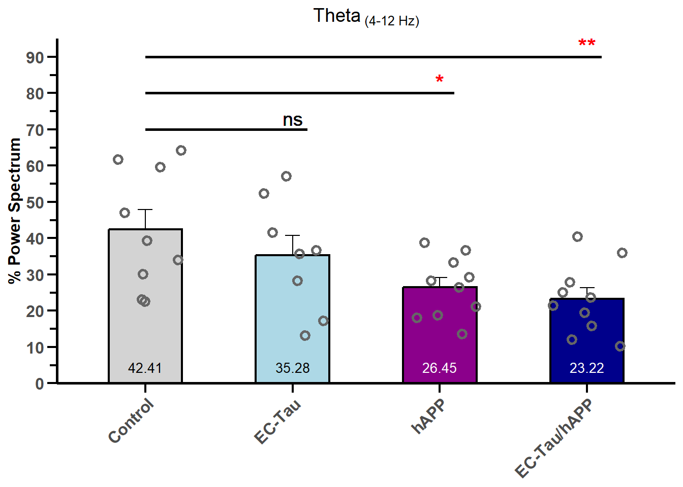
# save plot with white background
ggsave("LH_gamma.png", width=4, height=5, dpi=300, bg="white")